Neural Networks Explained: A Beginner's Guide

Introduction to Neural Networks

What are Neural Networks?

Neural Networks, also known as Artificial Neural Networks (ANNs), are computational systems inspired by the structure and function of the human brain. These networks are designed to recognize patterns, learn from data, and make decisions or predictions based on input data.

Key Characteristics:

• Neural Networks mimic the human brain's ability to learn and adapt.
• They consist of layers of interconnected nodes (neurons), where each connection is associated with a weight.

Brief History and Evolution

Neural Networks evolved as a response to the limitations of traditional computational systems and the increasing demand for intelligent systems capable of learning, adapting, and making complex decisions. Here’s an in-depth look into the reasons behind their evolution:

• Limitations of Rule-Based Systems: 

Early computational systems were largely rule-based, relying on explicitly programmed instructions to solve problems. These systems struggled with:

• Complexity: Writing rules for every scenario became unmanageable as tasks grew in complexity.
• Adaptability: Rule-based systems could not learn or adapt to new data.
• Pattern Recognition: Tasks like image recognition, speech processing, and language understanding required learning patterns, which rule-based systems couldn’t achieve effectively.

• Inspiration from the Human Brain:

The human brain is exceptionally good at:

• Learning from examples.
• Recognizing patterns in data.
• Making decisions in uncertain environments.

Researchers sought to mimic this biological intelligence by creating artificial systems modeled after the brain's structure and function. Neural Networks emerged as an abstraction of how neurons in the brain communicate and process information.

Biological Comparison:

• Biological Neuron: Dendrites (inputs) → Soma (processing) → Axon (output).
• Artificial Neuron: Inputs → Weights + Bias → Activation Function → Output.
• Increasing Availability of Data:

The evolution of Neural Networks coincided with the explosion of data due to:

• Internet Growth: Billions of daily searches, transactions, and interactions.
• Social Media: Platforms generating massive amounts of text, images, and videos.
• IoT Devices: Sensors producing real-time data streams.

This abundance of data created opportunities for systems capable of learning directly from vast datasets.

• Advances in Hardware

The introduction of key algorithms made Neural Networks practical and effective:

• Backpropagation (1986): Solved the problem of efficiently updating weights in multi-layer networks.
• Optimization Algorithms: Stochastic Gradient Descent (SGD), Adam, and RMSprop made training faster and more robust.
• Activation Functions: Functions like ReLU helped networks avoid vanishing gradients and learn complex patterns.

• Advances in Algorithms

The introduction of key algorithms made Neural Networks practical and effective:

• Backpropagation (1986): Solved the problem of efficiently updating weights in multi-layer networks.
• Optimization Algorithms: Stochastic Gradient Descent (SGD), Adam, and RMSprop made training faster and more robust.
• Activation Functions: Functions like ReLU helped networks avoid vanishing gradients and learn complex patterns.

• Real-World Problems Requiring Smarter Systems

Many real-world problems are too complex for traditional algorithms but are naturally suited for Neural Networks:

• Image Recognition: Identifying objects and faces in images.
• Speech Recognition: Translating spoken language into text.
• Natural Language Processing (NLP): Understanding, generating, and translating human language.

• Success Stories Driving Adoption

Successes in various fields solidified the importance of Neural Networks:

• ImageNet Challenge (2012): AlexNet, a deep convolutional network, dramatically reduced error rates in image classification.
• AlphaGo (2016): Demonstrated the ability of Neural Networks to master complex strategy games like Go.
• ChatGPT (2020s): Revolutionized conversational AI with large language models.

‍

Neural Networks are the foundation of deep learning, a subset of machine learning that has revolutionized various fields such as Disease diagnosis using medical imaging, Drug discovery and genomics, Personalized treatment recommendations, Fraud detection, Risk assessment, Algorithmic trading, Movie and music recommendation systems, Content creation using GANs, Autonomous driving, Traffic management, Adaptive learning systems, Automatic grading and tutoring.

Also Read: How Can We Shape the Future of Open-Source Intelligence?

The Inspiration Behind Neural Networks

The idea of Neural Networks emerged from a desire to replicate the learning and problem-solving capabilities of the human brain. Here’s a detailed exploration of what inspired their development:

Biological Inspiration: The Human Brain

The human brain is a complex network of approximately 86 billion neurons interconnected by trillions of synapses. Its remarkable abilities include:

• Learning from Experience: The brain adapts and rewires itself based on experiences, a process called neuroplasticity.
• Pattern Recognition: It excels in identifying patterns, whether in images, sounds, or text.
• Parallel Processing: The brain processes multiple signals simultaneously, making it highly efficient.

Technological Inspiration

The brain's efficiency inspired engineers and scientists to create systems that mimic its operations. Key motivations include:

1. Learning from Data: Traditional algorithms required explicit instructions, but Neural Networks aimed to learn directly from data.
2. Generalization: The ability to make predictions on unseen data.
3. Nonlinear Problem Solving: Neural Networks can model complex, nonlinear relationships that other methods struggle to handle.

Historical Contributions

Several milestones in science and technology contributed to the evolution of Neural Networks:

1. McCulloch-Pitts Model (1943):some text
   • Proposed the first mathematical model of a neuron.
   • Used binary inputs and outputs to mimic basic neuron operations.
2. Perceptron (1958):some text
   • Frank Rosenblatt's model introduced learning by adjusting weights based on errors.
3. Hebbian Learning (1949):some text
   • Inspired by biological learning, it emphasized strengthening connections between frequently co-activated neurons.
4. Backpropagation (1986):some text
   • Revolutionized Neural Networks by enabling efficient training of multi-layer networks.

Why Mimic the Brain?

• Universality: The brain’s principles are universal, applicable across vision, language, and reasoning tasks.
• Efficiency: Its structure allows for scalable, parallel computation.
• Robustness: The brain handles noisy and incomplete data effectively.

Key Components of a Neural Network

A neural network is built upon fundamental components that work together to process data and learn patterns. The neurons, often referred to as nodes, are the basic units that receive inputs, apply a weighted sum and bias, and pass the result through an activation function to determine the output. These neurons are organized into layers: the input layer, which accepts raw data; hidden layers, where computations and pattern extraction occur; and the output layer, which produces predictions or classifications. Weights and biases adjust the influence of inputs on the output, while the loss function measures the network’s performance. Learning is achieved through backpropagation, which optimizes weights and biases using gradient descent to minimize the loss, allowing the network to improve over time. These components collectively enable neural networks to solve a wide range of complex problems. Now let’s try to understand all these components in depth.

The Architecture of Neural Networks

The architecture of a neural network determines its structure, which consists of layers of interconnected neurons. These layers process data step by step, transforming inputs into meaningful outputs. Neural network architecture typically includes three main types of layers such as input layer, hidden layer and the output layer.

Neurons and Layers in Neural Networks

To understand how Neural Networks work, it’s essential to break down their fundamental building blocks. Every Neural Network consists of components that collaborate to process data, learn patterns, and make predictions. In Neural Networks, neurons and layers work together to process inputs, learn from data, and make predictions. Understanding their interplay is crucial for mastering Neural Networks.

Here's an in-depth explanation of these key components:

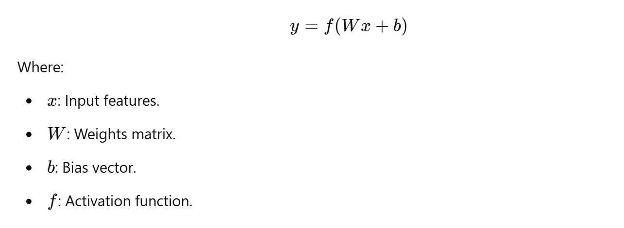
Neurons: The Basic Processing Units

Neurons, also called nodes or units, are the smallest computational units in a Neural Network.

Each neuron receives inputs, processes them by applying weights, biases, and an activation function, and then passes the result to the next layer and produces an output.

It Mimics the biological neuron by integrating inputs and producing a signal based on the threshold.

‍

Mathematics Behind a Neuron

Example:

‍

Layers: Organizing Neurons

Neurons are organized into layers, with each layer performing a specific task in the learning process.

Input Layer

Accepts raw data and passes it to the network. Each neuron in this layer represents a feature of the input data. Each neuron in the input layer corresponds to one feature or input dimension.

‍

Hidden Layers

It extracts and learns patterns or features from the input. Process data using learned weights and biases to identify patterns and relationships. It can have multiple layers (Deep Neural Networks). The number of neurons and layers affects the network's capacity to learn complex patterns. Each neuron connects to all neurons in the previous and next layers (fully connected layers). More layers (Depth) enables the network to learn complex, hierarchical features (e.g., detecting edges, shapes, and objects in images). Fewer layers are suitable for simpler problems.

Output Layer

Produces the final result or prediction. The number of neurons corresponds to the number of classes or outputs. For example, In a binary classification, the output layer has one neuron with a sigmoid activation function.

Connections Between Neurons

Weights, biases, and activation functions form the backbone of Neural Networks. They determine how data flows through the network and enable the model to learn patterns and relationships in the data. Let’s explore these components in detail.

Weights (w)

Weights are the coefficients that determine the importance of each input. High weights amplify the input signal, while low weights suppress it. It determines the strength of the connection between neurons in adjacent layers. It amplifies or diminishes the influence of an input. Weights allow the network to focus on important features during training. The weights are adjusted during training using optimization algorithms like Gradient Descent.

Bias (b)

Bias is a constant added to the weighted sum. It shifts the activation function, enabling the model to better fit the data. It allows neurons to activate even if the weighted sum is zero.

Mathematical Representation:

Activation Functions

Activation functions introduce non-linearity, enabling the network to learn complex patterns. It converts the weighted sum into a meaningful output and decides whether a neuron should activate or not.

‍

Types of Activation Functions:

Activation functions introduce non-linearity into neural networks, enabling them to model complex relationships in data. Each activation function has unique properties that make it suitable for specific tasks.

‍

1. Linear Activation Function

Equation: 

‍

Characteristics:

• Directly outputs the input as the activation.
• No non-linearity: It cannot model complex data relationships.
• Derivative is constant, which simplifies optimization but limits learning.

Use Case:

Rarely used in hidden layers but sometimes in the output layer for regression problems.

‍

2. Sigmoid Activation Function

Equation:

Characteristics:

• Output range: [0,1].
• S-shaped (sigmoidal) curve.
• Converts large input values to values close to 1 and small values to values close to 0.

Pros:

• Good for binary classification.
• Smooth gradient, preventing abrupt changes during optimization.

Cons:

• Vanishing Gradient Problem: Gradients become very small for large or small zzz, slowing learning.
• Outputs are not zero-centered, causing inefficiency during optimization.

Graph:

The sigmoid curve flattens as z approaches extreme values, showing the saturation effect.

‍

Use Case:

• Binary classification (e.g., predicting if an email is spam or not).

‍

3. Tanh (Hyperbolic Tangent) Activation Function

Equation:

‍

Characteristics:

• Output range:[−1,1].
• S-shaped curve similar to sigmoid but zero-centered.

Pros:

• Zero-centered outputs simplify optimization.
• Can handle negative input values better than sigmoid.

Cons:

• Suffers from the vanishing gradient problem for large or small zzz.

Graph:

The Tanh curve is similar to Sigmoid but shifts the range to [−1,1], making it more balanced.

Use Case:

• Often used in RNNs where zero-centered outputs are helpful.

4. ReLU (Rectified Linear Unit) Activation Function

Equation:

Characteristics:

• Outputs z for z>0; otherwise, outputs 0.
• Introduces sparsity, as many neurons output 0 (inactive).

Pros:

• Computationally efficient.
• No vanishing gradient problem for z>0.
• Works well in deep networks.

Cons:

• Dead Neurons Problem: Neurons may output 0 for all inputs, effectively dying.
• Not differentiable at z=0 (though this is rarely an issue in practice).

Graph:

The ReLU curve is linear for z > 0 and flat for z ≤ 0.

Use Case:

• Most commonly used in hidden layers of deep networks.

‍

5. Leaky ReLU Activation Function

Equation:

Characteristics:

• Variant of ReLU with a small slope (α) for z ≤ 0.

Pros:

• Solves the dead neuron problem.
• Retains computational efficiency.

Cons:

• Introduces an additional parameter (α).

Graph:

Similar to ReLU, but the negative part has a slight slope.

Use Case:

• Alternative to ReLU when dead neurons are problematic.

6. Softmax Activation Function

Equation:

Characteristics:

• Converts logits into probabilities that sum to 1.
• Typically used in the output layer for multi-class classification.

Pros:

• Provides interpretable probability outputs.
• Ensures outputs are mutually exclusive.

Cons:

• Computationally expensive for large output spaces.

Graph:

The Softmax function doesn’t have a direct graph, as it maps a vector of logits to a vector of probabilities.

Use Case:

• Multi-class classification problems (e.g., classifying handwritten digits).

‍

The graph above represents the popular six activation functions. Here's what each subplot illustrates:

1. Linear: The output directly corresponds to the input, with no transformation.
2. Sigmoid: A smooth curve that maps input values to the range [0, 1].
3. Tanh: A zero-centered activation function with an output range of [-1, 1].
4. ReLU: Outputs positive inputs as they are and sets negative inputs to zero.
5. Leaky ReLU: Similar to ReLU but allows a small slope for negative inputs to address the dead neuron problem.
6. Softmax: Normalizes input values into probabilities, but for clarity in this graph, it appears as a smoothed transformation.

Also Read: How Artificial Intelligence Automation is Revolutionizing Sales Processes

Forward Propagation: How Neural Networks Make Predictions

Now that we’ve discussed the foundational components of neural networks—including neurons, layers, weights, biases, and activation functions—let’s move to the next logical step: forward propagation. This is the process where input data flows through the network, layer by layer, to produce an output. It’s the forward “path” that transforms raw data into predictions, leveraging the components we’ve already explored.

What is Forward Propagation?

Forward propagation is the core computation that happens when a neural network is used to make predictions. During this process, the input data:

1. Passes through the input layer.
2. Undergoes transformations in the hidden layers.
3. Produces an output via the output layer.

These transformations are a combination of linear operations (weighted sums and biases) and non-linearities introduced by activation functions. The network’s ability to learn complex patterns stems from this blend of linear and non-linear operations.

‍

The Mathematical Journey of Forward Propagation

Step 1: From Input Layer to First Hidden Layer

The neurons in the hidden layer take the input features, multiply them by their respective weights, add biases, and pass the result through an activation function:

Step 2: From Hidden Layers to Subsequent Layers

For each hidden layer, the same computations are repeated. The output of one layer serves as the input for the next:

Step 3: From Last Hidden Layer to Output Layer

The final layer transforms the last hidden layer's activations into outputs. For classification tasks, the activation function might be softmax (for probabilities) or sigmoid (for binary outputs):

For example imagine you’re building a neural network to classify handwritten digits (e.g., MNIST dataset). For a given image:

1. The input layer receives pixel values (flattened into a vector).
2. The hidden layers compute patterns, such as edges or shapes, by applying weights, biases, and activations.
3. The output layer assigns probabilities to each digit class (0–9) using the softmax activation.

Forward propagation involves both linear transformations and non-linear activation functions. Each layer’s output feeds into the next, allowing the network to capture increasingly complex patterns. The activation functions, as we discussed earlier, introduce non-linearity, enabling the network to model non-linear relationships in the data.

Also Read:  How Artificial Intelligence is Revolutionizing Various Industries

The Role of Loss Functions in Neural Networks

Loss functions are critical in training neural networks as they measure the difference between the network’s predictions and the actual target values. A loss function provides a quantitative value that guides the learning process—lowering the loss implies improving the model’s predictions. By minimizing this loss during training, the network learns to generalize better and make more accurate predictions.

Why Loss Functions Are Essential

1. Guiding Training: Loss functions determine how well or poorly the neural network is performing.
2. Optimization: They are essential for adjusting weights and biases during backpropagation.
3. Feedback Mechanism: The loss provides feedback to the optimizer, which uses it to tweak the model parameters.
4. Adaptability: Different tasks (classification, regression, etc.) require different loss functions tailored to their specific needs.

Types of Loss Functions

1. Loss Functions for Regression

Loss functions for regression tasks measure the numerical distance between predicted and actual values.

Mean Squared Error (MSE):

Measures the average of the squared differences between predicted values( y hat_i) and actual values (y_i).

Formula: 

Properties:

• Penalizes larger errors more than smaller ones.
• Sensitive to outliers.

Mean Absolute Error (MAE):

Measures the average of the absolute differences between predicted and actual values.

Formula: 

Properties:

• Treats all errors equally.
• Less sensitive to outliers.

2. Loss Functions for Classification

Loss functions for classification evaluate how well the predicted probabilities match the true classes.

Cross-Entropy Loss:

• Widely used for multi-class classification.
• Measures the distance between the predicted probability distribution(y hat i) and the true distribution (y).

Formula: 

Properties:

Penalizes incorrect predictions with higher confidence.

‍

Binary Cross-Entropy:

• A special case of cross-entropy for binary classification.

Formula:

3. Special Loss Functions

Hinge Loss:

Used for binary classification, especially with Support Vector Machines (SVMs).

Formula:

Huber Loss:

A hybrid of MSE and MAE, robust to outliers.

Formula:

Choosing the Right Loss Function

The selection of a loss function depends on the problem:

• Regression: Use MSE or MAE.
• Binary Classification: Use Binary Cross-Entropy.
• Multi-class Classification: Use Cross-Entropy.

Backpropagation and Gradient Descent: How Neural Networks Learn

Backpropagation and gradient descent are the backbone of a neural network's learning process. They work together to adjust the model's weights and biases iteratively, enabling the network to minimize the error and improve performance over time.

Backpropagation: Understanding the Core Mechanism

Backpropagation (short for "backward propagation of errors") is a supervised learning algorithm used to train neural networks. It calculates the gradient of the loss function with respect to each weight by applying the chain rule of calculus.

Steps in Backpropagation

1. Forward Propagation:some text
   • Input data passes through the network.
   • Predictions (y hat​) are generated at the output layer.
2. Loss Calculation:some text
   • The loss function computes the error between the predicted values (y hat​) and actual values (y).
3. Backward Propagation:some text
   • Errors are propagated backward through the network.
   • Gradients of the loss function are calculated with respect to weights and biases using the chain rule.
4. Weight and Bias Updates:some text
   • The calculated gradients are used to adjust the network's parameters to minimize the loss.

Gradient Descent: Optimization in Action

Gradient descent is an optimization algorithm used to minimize the loss function. It updates weights and biases in the direction of the steepest descent of the loss function.

Gradient Descent Formula

For a weight w:

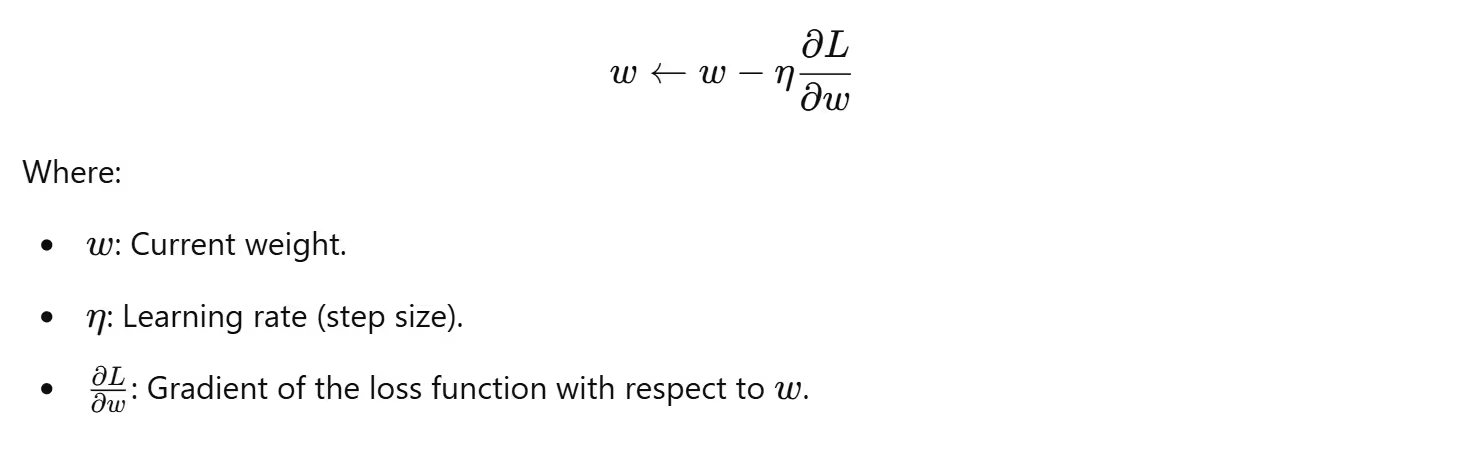
Mathematical Intuition

Chain Rule in Backpropagation

To calculate the gradient of the loss function L with respect to weights in earlier layers:

Gradient Calculation

For a neuron:

Types of Gradient Descent

1. Batch Gradient Descent:some text
   • Updates weights using the entire dataset.
   • Slow but accurate.
2. Stochastic Gradient Descent (SGD):some text
   • Updates weights using a single data point.
   • Faster but noisier.
3. Mini-Batch Gradient Descent:some text
   • Updates weights using a subset of the dataset.
   • Balances speed and accuracy.

Challenges in Backpropagation

1. Vanishing Gradient: Gradients become too small, slowing down learning for deeper layers.
2. Exploding Gradient: Gradients grow too large, leading to unstable updates.
3. Learning Rate Sensitivity: A learning rate that's too high can cause divergence, while one that's too low slows down learning.

Backpropagation and gradient descent are the backbone of neural network learning. Understanding their mechanics is crucial for designing and optimizing neural networks effectively. 

‍

How Neural Networks Learn

Neural networks learn by optimizing their parameters—weights and biases—to minimize the error between the predicted output and the actual target. This learning process involves a cycle of data passing through the network, error calculation, and parameter adjustment.

How Learning Happens

1. Data Flow Through the Network (Forward Propagation):some text
   • Input data is transformed layer by layer using weights, biases, and activation functions.
   • The output at the final layer is the network's prediction.
2. Error Measurement (Loss Function):some text
   • The difference between the predicted output and the actual target is calculated using a loss function.
   • For example:some text
     • Mean Squared Error (MSE) for regression tasks.
     • Cross-Entropy Loss for classification tasks.
3. Error Signal Propagation (Backward Propagation):some text
   • The error signal is propagated backward through the network.
   • Gradients of the loss function with respect to weights and biases are calculated using the chain rule of calculus.
4. Parameter Update (Optimization):some text
   • The gradients are used to adjust the weights and biases in the direction that reduces the loss.
   • Gradient descent (or its variants) is the algorithm typically used for this step.

Key Concepts in Learning

Epochs, Batches, and Iterations:

• Epoch: One complete pass through the entire dataset.
• Batch: A subset of the dataset used for one forward and backward pass.
• Iteration: One update step, typically for one batch.

Learning Rate:

• Controls the size of each update step.
• A small learning rate ensures slow but steady convergence.
• A large learning rate can lead to overshooting the minimum or divergence.

Regularization:

• Techniques like L1, L2 regularization, and dropout prevent overfitting by penalizing large weights or randomly dropping units during training.

Early Stopping:

• Stops training once the performance on a validation set stops improving, avoiding overfitting.

Mathematical Intuition

For a single neuron:

1. Compute the weighted sum of inputs and bias:

2. Apply the activation function:

3. Update the weights using the gradient of the loss:

For a multilayer network, the process is extended to all layers, propagating gradients backward during backpropagation.

Neural networks learn through a systematic process of forward propagation, error measurement, backward propagation, and parameter updates. By iteratively refining their parameters, they achieve remarkable accuracy in making predictions for diverse tasks.

The Role of Gradients and Learning Rates

In neural networks, the role of gradients and learning rates is critical in determining how efficiently and effectively the model learns from the data. Gradients guide the direction of parameter updates, while the learning rate controls the step size in that direction. Together, they govern the convergence behavior of the model during training.

What Are Gradients?

Gradients are partial derivatives of the loss function with respect to the model parameters (weights and biases). They represent the slope of the loss function in parameter space and indicate how much a change in parameters will affect the loss.

Mathematical Representation:

The sign of the gradient determines the direction to move:

• Positive gradient: Decrease www to reduce loss.
• Negative gradient: Increase www to reduce loss.

The Role of Learning Rate

The learning rate (η) is a hyperparameter that scales the magnitude of parameter updates during gradient descent. It controls how quickly the model learns:

Choosing the Right Learning Rate:

1. Too Small:some text
   • Slow convergence.
   • Prolonged training time.
2. Too Large:some text
   • Risk of overshooting the optimal point.
   • Possible divergence.

Adaptive Learning Rates:

Modern optimizers like Adam and RMSprop dynamically adjust the learning rate during training for better performance.

Gradients and learning rates form the backbone of the training process in neural networks. Understanding their interplay is crucial for designing models that converge efficiently and accurately. By fine-tuning these components, we can optimize the learning process and achieve better results.

Types of Neural Networks 

Neural networks have evolved into diverse architectures, each tailored to specific problem domains and data structures. This section delves into the most common types, their architectures, how they work, and their real-world applications.

‍

1. Feedforward Neural Networks (FNNs)

Description:

• Also called dense or fully connected networks.
• Data flows in one direction, from the input to the output layer, without cycles or loops.
• Form the foundation of neural networks and are used for tasks where the input and output have no inherent sequential relationship.

Architecture:

• Input Layer: Accepts raw input features.
• Hidden Layers: Intermediate layers where transformations occur using weights, biases, and activation functions.
• Output Layer: Produces the final prediction or output.

Mathematics:

The prediction is computed as:

Applications:

• Predicting stock prices.
• Diagnosing diseases.
• Handwriting and speech recognition.

Here’s a simple code example to create an Artificial Neural Network (ANN) using TensorFlow/Keras. This example uses the famous Iris dataset for training and testing. The goal is to classify the iris flower into one of three species based on its features.

‍

2. Convolutional Neural Networks (CNNs)

Description:

• Specialized for processing grid-like data, such as images or videos.
• Employ convolution operations to detect patterns (edges, textures) in spatially organized data.
• Use shared weights (kernels) to reduce the number of parameters and improve generalization.

Architecture:

1. Convolutional Layers:some text
   • Apply filters (kernels) over input data.
   • Output feature maps highlight specific patterns.
2. Pooling Layers:some text
   • Downsample feature maps to reduce dimensions and computational complexity.
   • Example: Max pooling selects the maximum value in a region.
3. Fully Connected Layers:some text
   • Flatten feature maps and connect neurons to perform the final classification.

Mathematics:

Convolution operation:

Applications:

• Image classification (e.g., cats vs. dogs).
• Object detection (e.g., autonomous vehicles).
• Medical imaging (e.g., tumor detection).

3. Recurrent Neural Networks (RNNs)

Description:

• Designed for sequential data where order matters, such as time series or natural language.
• Use hidden states to retain information from previous inputs, enabling temporal learning.

Architecture:

• Input Layer: Receives sequential data.
• Recurrent Layers: Include loops to store and propagate temporal information.
• Output Layer: Produces predictions for each time step or the entire sequence.

Mathematics:

The hidden state at time t is:

Challenges:

• Vanishing Gradient Problem: Gradients diminish over time steps, making it hard to learn long-term dependencies.

Variants:

• LSTMs (Long Short-Term Memory):some text
  • Use gates (input, forget, output) to manage information flow.
• GRUs (Gated Recurrent Units):some text
  • Simplified version of LSTMs with fewer gates.

Applications:

• Machine translation (e.g., English to French).
• Speech recognition.
• Stock price prediction.

4. Generative Adversarial Networks (GANs)

Description:

• Consist of two networks, a generator and a discriminator, that compete against each other.
• The generator creates data, and the discriminator evaluates its authenticity.
• Both networks improve iteratively, producing high-quality synthetic data.

Architecture:

1. Generator:some text
   • Takes random noise as input.
   • Produces data resembling the target distribution.
2. Discriminator:some text
   • Distinguishes between real and synthetic data.
   • Provides feedback to the generator.

Mathematics:

Objective function:

Applications:

• Image generation (e.g., Deepfake creation).
• Super-resolution.
• Data augmentation for training.

‍

5. Specialized Architectures

Autoencoders:

• Unsupervised models for encoding data into latent spaces.
• Applications: Noise reduction, anomaly detection, data compression.

Transformers:

• Replace RNNs for sequential tasks using self-attention mechanisms.
• Applications: Language translation, text summarization (e.g., GPT, BERT).

Spiking Neural Networks (SNNs):

• Inspired by the brain's neurons.
• Suitable for neuromorphic computing and real-time edge processing.

The diversity of neural network types highlights their adaptability across domains. By selecting the appropriate architecture based on the problem and data characteristics, you can harness the power of neural networks to achieve remarkable results in real-world applications.

Common Applications of Neural Networks

Neural networks have revolutionized numerous industries, offering state-of-the-art solutions to complex problems. Their ability to model non-linear relationships, learn patterns, and make predictions has paved the way for advancements across diverse domains. Below, we explore key applications with explanations and examples.

1. Image Recognition

Neural networks, particularly Convolutional Neural Networks (CNNs), have excelled in image recognition tasks by identifying and classifying objects, patterns, and features in images.

Examples:

• Facial Recognition: Security systems use neural networks to match facial features.
• Medical Imaging: Detecting tumors or abnormalities in X-rays and MRIs.
• Object Detection: Applications in autonomous vehicles to detect road signs, pedestrians, and obstacles.

Case Study:

• Google Photos uses CNNs for automatic photo categorization, tagging, and searching by recognizing objects and faces.

2. Natural Language Processing (NLP)

Recurrent Neural Networks (RNNs), Transformers, and variants like GPT and BERT have brought breakthroughs in understanding and generating human language.

Examples:

• Sentiment Analysis: Analyzing customer feedback or social media sentiment.
• Machine Translation: Converting text from one language to another (e.g., Google Translate).
• Text Summarization: Generating concise summaries of lengthy documents or articles.

Case Study:

• OpenAI's GPT models power applications like ChatGPT, enabling context-aware conversational AI systems.

3. Speech Recognition

Neural networks process and interpret audio signals to transcribe speech into text or recognize spoken commands.

Examples:

• Voice Assistants: Alexa, Google Assistant, and Siri use neural networks for speech-to-text and intent recognition.
• Call Centers: Automating customer service interactions.

Mathematics:

Spectrogram analysis via neural networks maps audio signals to linguistic representations.

4. Autonomous Vehicles

Neural networks play a crucial role in enabling self-driving cars by processing data from sensors, cameras, and LiDAR.

Tasks:

• Object Detection: Identifying cars, pedestrians, and traffic signs.
• Path Planning: Predicting safe trajectories.
• Decision Making: Navigating intersections and handling dynamic traffic scenarios.

Case Study:

• Tesla’s Autopilot uses a combination of CNNs and RNNs for real-time vehicle control.

5. Healthcare

Neural networks assist in diagnostics, treatment planning, and drug discovery by analyzing medical data.

Examples:

• Disease Detection: Identifying diabetes or cancer from patient records.
• Drug Development: Predicting molecular interactions for new medicines.
• Personalized Medicine: Tailoring treatments based on genetic data.

Case Study:

• IBM Watson Health uses neural networks to provide insights for oncologists in cancer treatment.

Also Read: How AI in Healthcare Industry Is Driving New Trends ?

6. Finance

Neural networks help in predicting market trends, detecting fraud, and optimizing financial portfolios.

Examples:

• Stock Market Prediction: Analyzing historical data for investment decisions.
• Fraud Detection: Identifying anomalous transactions in banking systems.
• Credit Scoring: Assessing customer creditworthiness.

7. Generative Models

Generative Adversarial Networks (GANs) and Variational Autoencoders (VAEs) create new data based on learned patterns.

Examples:

• Image Generation: Producing realistic images (e.g., Deepfakes).
• Content Creation: Generating music, art, and text.
• Data Augmentation: Synthesizing training data for machine learning tasks.

Case Study:

• NVIDIA’s GauGAN generates lifelike images from simple sketches.

8. Gaming

Neural networks enhance gaming experiences by creating adaptive AI and realistic graphics.

Examples:

• Game AI: Non-player characters (NPCs) learn and adapt to player behavior.
• Graphics: Enhancing realism through super-resolution techniques.

Case Study:

• AlphaGo, developed by DeepMind, defeated human champions in the board game Go using reinforcement learning.

9. Recommendation Systems

Neural networks analyze user preferences and behavior to provide personalized recommendations.

Examples:

• E-commerce: Suggesting products on Amazon.
• Entertainment: Recommending movies on Netflix or songs on Spotify.
• Social Media: Curating posts and advertisements based on user interests.

10. Predictive Maintenance

Neural networks monitor equipment performance to predict failures and optimize maintenance schedules.

Examples:

• Manufacturing: Predicting machinery breakdowns.
• Aviation: Monitoring aircraft engines to prevent failures.

Case Study:

• GE Aviation uses neural networks to analyze engine data for proactive maintenance.

Neural networks are transforming industries by enabling innovative solutions across domains. Understanding these applications not only illustrates the versatility of neural networks but also inspires new ways to leverage their potential.

Conclusion

Neural networks have emerged as a cornerstone of modern artificial intelligence, providing solutions to problems once considered insurmountable. As we wrap up this guide, it’s essential to reflect on the journey so far and explore future possibilities.

Neural networks are not just a technological innovation and check out the blog how Artificial Intelligence is Revolutionizing Various Industries; they are a tool for shaping the future. Whether you’re a beginner taking your first steps or an expert pushing the boundaries, the journey of mastering neural networks is as rewarding as it is challenging. Embrace the concepts, experiment fearlessly, and join the ever-growing community of AI enthusiasts driving the next wave of innovation.

"The best way to predict the future is to create it." — Abraham Lincoln

‍