Principal Component Analysis (PCA): Simplifying Data Without Losing Insights

Introduction to PCA

Principal Component Analysis (PCA) is one of the most widely used techniques in machine learning and statistics for dimensionality reduction. It simplifies complex datasets by transforming them into a smaller number of dimensions while retaining as much variability as possible. PCA helps to uncover hidden patterns, relationships, or structures in high-dimensional data.

In essence, PCA converts the original data into a new coordinate system where the axes (principal components) represent the directions of maximum variance. By focusing on the most significant components, we can reduce the number of features in a dataset without losing critical insights.

For example, consider a dataset with hundreds of features. Visualizing or analyzing this dataset directly can be challenging due to its complexity. PCA helps by reducing the dimensions to two or three, making it easier to visualize, interpret, and build machine learning models.

Why is PCA Important?

• High-dimensional datasets can be noisy and computationally expensive to process.
• PCA reduces redundancy in data by focusing on variability.
• It helps avoid overfitting in machine learning models by eliminating irrelevant or less important features.
• PCA is not just a tool for data reduction but also a means to better understand the underlying structure of the data.

Also Read: The Differences Between Neural Networks and Deep Learning Explained

The Need for Dimensionality Reduction in Machine Learning

In today’s era of big data, machine learning models often deal with datasets containing hundreds or even thousands of features. While high-dimensional data may provide rich information, it also introduces several challenges, making dimensionality reduction techniques like PCA essential.

Challenges Posed by High-Dimensional Data

1. The Curse of Dimensionality
   
   
   
   • As the number of features increases, the data becomes sparse, making it harder for models to find meaningful patterns.
   • Distance metrics used in algorithms like k-Nearest Neighbors (k-NN) lose their effectiveness in high dimensions.
2. Increased Computational Complexity
   
   
   
   • More features mean higher memory requirements and longer training times.
   • Algorithms, especially those with quadratic or exponential complexity, struggle to scale with the number of features.
3. Overfitting
   
   
   
   • High-dimensional datasets can cause models to overfit by learning noise instead of generalizable patterns.
   • Reducing dimensions helps focus on the most important features, improving model generalization.
4. Difficulty in Visualization
   
   
   
   • Human interpretation of data beyond three dimensions is impossible.
   • Dimensionality reduction simplifies datasets, making it easier to visualize relationships and trends.

How Dimensionality Reduction Helps

1. Improved Model Performance
   
   
   
   • By removing redundant and less relevant features, dimensionality reduction ensures that the model focuses on the most impactful data points, often improving accuracy.
2. Noise Reduction
   
   
   
   • Dimensionality reduction filters out noise by identifying and preserving the features that contribute the most to variance in the data.
3. Better Interpretability
   
   
   
   • A smaller set of features is easier to understand and explain, especially in applications where interpretability is critical (e.g., healthcare, finance).
4. Enabling Visualization
   
   
   
   • PCA and similar techniques reduce complex datasets into 2 or 3 dimensions, enabling clear visual representations like scatter plots.

Real-World Scenarios Highlighting the Need

• Genomics: Datasets with thousands of genes make analysis complex. PCA helps identify key gene expressions related to diseases.
• Marketing: Customer datasets with hundreds of features can be simplified to focus on major purchasing behaviors.
• Image Processing: High-resolution images contain millions of pixels. PCA reduces dimensions while retaining key visual features.

By addressing these challenges, PCA and other dimensionality reduction techniques play a pivotal role in simplifying data analysis while preserving valuable insights.

Also Read: Building and Implementing Effective NLP Models with Transformers

Mathematical Foundations of PCA

To understand Principal Component Analysis (PCA), it’s essential to grasp the mathematical concepts behind it. PCA uses linear algebra to transform a high-dimensional dataset into a new coordinate system, where the new axes (called principal components) capture the maximum variance in the data.

Key Concepts Behind PCA

1. Variance: Variance measures the spread of data points around the mean. PCA identifies directions in the data (principal components) that have the maximum variance, as these directions capture the most significant information.
2. Covariance: Covariance quantifies how two variables vary together. The covariance matrix is central to PCA, as it identifies relationships between variables in the dataset.
3. Linear Transformation: PCA transforms the data into a new space defined by linear combinations of the original features, with each new axis (principal component) being orthogonal to the others.

‍

Steps in the Mathematical Process of PCA

1. Standardize the Data:
   
   
   
   • Data must be scaled so that features with larger ranges don’t dominate the analysis.
   • This is done by subtracting the mean and dividing by the standard deviation for each feature.

 Where zij is the standardized value, xij is the original data point, μj is the mean, and σj is the standard deviation of feature j.

2. Compute the Covariance Matrix:
   
   
   
   • The covariance matrix captures pairwise relationships between variables.
   • For a dataset X with n features, the covariance matrix C is:

Each entry cij represents the covariance between feature ii and feature j.

3. Calculate Eigenvalues and Eigenvectors:
   
   
   
   • Eigenvalues represent the amount of variance captured by each principal component.
   • Eigenvectors define the directions of the principal components.
   • Solve the equation:

Where A is the covariance matrix, λ (eigenvalues) represents the variance along the eigenvector v.

4. Sort and Select Principal Components:
   
   
   
   • Arrange eigenvalues in descending order and select the top kk components that capture the most variance.
5. Project Data onto the New Subspace:
   
   
   
   • Transform the original dataset into the lower-dimensional space using the eigenvectors:

Where Z is the transformed data, X is the original data, and W is the matrix of selected eigenvectors.

Intuition Behind the Mathematics

Imagine PCA as finding a new coordinate system for the data. This system is oriented such that:

• The first axis (principal component) captures the maximum variance in the data.
• The second axis is orthogonal to the first and captures the next highest variance, and so on.

By focusing on the axes with the most variance, PCA effectively simplifies the data while retaining its essential structure.

Also Read: Data Preprocessing in Machine Learning: A Guide to Cleaning and Preparing Data

Variance and Covariance

Understanding variance and covariance is crucial to grasping how PCA works, as these concepts form the basis of the covariance matrix used in PCA.

‍

What is Variance?

Variance measures the spread of data points around their mean. A higher variance indicates that the data points are more spread out, while a lower variance suggests they are closer to the mean.

The formula for variance of a single variable X is:

Where:

• xi: Individual data points
• μ: Mean of the data
• n: Number of data points

In PCA, variance is crucial because the principal components are chosen based on the directions that maximize variance.

‍

What is Covariance?

Covariance quantifies the relationship between two variables. It indicates whether changes in one variable are associated with changes in another. If the covariance is:

• Positive: Both variables increase or decrease together.
• Negative: One variable increases as the other decreases.
• Zero: The variables are independent of each other.

The formula for covariance between two variables X and Y is:

Where:

• μX and μY: Means of variables X and Y.
• xi,yi: Individual data points for X and Y.

Also Read: How to Build Your First Convolutional Neural Network: A Step-by-Step Guide

Covariance Matrix

For datasets with multiple variables, PCA uses the covariance matrix to analyze relationships between all pairs of variables. The covariance matrix is a square, symmetric matrix where each entry represents the covariance between two variables.

For a dataset X with nn variables, the covariance matrix C is:

Variance and Covariance in PCA

• Variance: Principal components are oriented in the directions of maximum variance. The first principal component captures the largest variance in the data, the second the next largest, and so on.
• Covariance: The covariance matrix tells us how variables are correlated. PCA uses this matrix to compute eigenvalues and eigenvectors, which define the principal components.

‍

Example

Consider a dataset with two features, Height (X) and Weight (Y):

1. Compute the mean of X and Y.
2. Calculate the variance of each feature.
3. Compute the covariance between X and Y.
4. Construct the covariance matrix:

Let me know if you'd like a detailed calculation example for the dataset or if you'd like me to move on to the next section!

Eigenvalues and Eigenvectors

Eigenvalues and eigenvectors are the mathematical backbone of PCA. They are derived from the covariance matrix and help identify the principal components, which are the directions of maximum variance in the data.

What are Eigenvalues and Eigenvectors?

1. Eigenvector:
   
   
   
   • A nonzero vector that remains in the same direction (scaled) when a linear transformation (like applying the covariance matrix) is applied to it.
   • It represents the direction of a principal component in PCA.
2. Eigenvalue:
   
   
   
   • A scalar value associated with an eigenvector.
   • It indicates the magnitude of variance captured by the eigenvector (i.e., how "important" that direction is).

Mathematically, eigenvalues and eigenvectors are derived from the covariance matrix CC by solving the equation:

Where:

• C: Covariance matrix
• v: Eigenvector
• λ: Eigenvalue

Also Read: How to Learn Coding at Home: A Beginner’s Guide to Self-Taught Programming

Role of Eigenvalues and Eigenvectors in PCA

• Eigenvectors define the axes of the new feature space (principal components).
• Eigenvalues determine the amount of variance (or information) captured by each principal component. Larger eigenvalues correspond to more significant components.

‍

Step-by-Step Process to Compute Eigenvalues and Eigenvectors

1. Start with the Covariance Matrix C:
   Compute the covariance matrix of the standardized dataset.
   
   
2. Solve the Characteristic Equation:
   The characteristic equation is derived from:
   

1. 
   Where I is the identity matrix. Solving this equation gives the eigenvalues (λ\lambda).
   
   
2. Find the Eigenvectors:
   For each eigenvalue, solve:
   

1. 
   This gives the eigenvector vv corresponding to that eigenvalue.
   
   
2. Sort Eigenvalues and Eigenvectors:
   
   
   
   • Arrange eigenvalues in descending order.
   • The eigenvector associated with the largest eigenvalue becomes the first principal component, and so on.

Geometric Intuition

• Eigenvectors represent the directions (axes) along which the data varies the most.
• Eigenvalues quantify how much variance exists in the direction of each eigenvector.

For example, in a 2D dataset, eigenvectors might point along the major and minor axes of the data’s spread, and eigenvalues indicate the strength of the spread along these axes.

Connecting to PCA

1. Eigenvalues (λ=3,1) indicate the amount of variance along the corresponding eigenvectors.
2. Eigenvectors ([1,1] and [−1,1]) define the new axes (principal components).
3. The data is projected onto these axes to achieve dimensionality reduction.

Also Read: Uses of Artificial Intelligence: How AI is Revolutionizing Industries

The PCA Algorithm: Step-by-Step Breakdown

Principal Component Analysis (PCA) is performed through a structured sequence of steps, starting from preprocessing the data to projecting it onto the principal components. Here's a detailed breakdown of the PCA algorithm:

Step 1: Standardize the Data

• PCA is sensitive to the scale of variables. To ensure that variables with larger ranges do not dominate the analysis, standardize the dataset by converting it to have zero mean and unit variance.
• For each feature Xj, compute:

Where:

• μj: Mean of feature j
• σj: Standard deviation of feature j
• zj: Standardized value

‍

Step 2: Compute the Covariance Matrix

• Calculate the covariance matrix C for the standardized dataset.
• For a dataset X with nn features: 

Where m is the number of data points.

‍

Step 3: Calculate Eigenvalues and Eigenvectors

• From the covariance matrix C:
  
  • Compute eigenvalues (λ) and eigenvectors (v).
• Eigenvectors define the directions (principal components).
• Eigenvalues indicate the amount of variance captured by each principal component.

‍

Step 4: Sort Eigenvalues and Select Principal Components

• Sort eigenvalues in descending order along with their corresponding eigenvectors.
• Choose the top k eigenvectors (corresponding to the k largest eigenvalues) to form a new feature subspace.

If λ1,λ2,…,λk are the eigenvalues:

• The proportion of variance explained by each component is: 

‍

Step 5: Transform the Data

• Project the original dataset onto the selected principal components (eigenvectors).
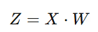
• The transformed dataset Z is computed as:

 Where W is the matrix of the top k eigenvectors.

‍

Step 6: Reconstruct the Data (Optional)

• If needed, reconstruct the original dataset using the principal components.
• The approximation is: 

‍

Illustrative Example

Let’s apply PCA to a 2D dataset with features X1 (height) and X2 (weight):

1. Dataset (Original Values):

2. Standardize the Data:

 Compute the mean and standard deviation for each feature, and standardize the dataset.

3. Covariance Matrix:
   Using the standardized data, calculate the covariance matrix C.
   
   
4. Eigenvalues and Eigenvectors:
   Compute eigenvalues and eigenvectors for C.
   For example:

5. Choose Principal Components:
   Select the eigenvector corresponding to λ1=3 (the component with maximum variance).
   
   
6. Transform the Data:
   Project the original data onto v1.
   
   

The PCA algorithm simplifies datasets by identifying key directions of variance (principal components) and projecting the data onto these directions. This reduces the number of features while retaining as much meaningful information as possible.

Also Read: How to Build an Effective Data Stack for Your Organization

Visualizing PCA: Understanding Principal Components

PCA is not just a mathematical tool but also a method that can be visualized to gain a deeper understanding of the data and the principal components. Visualizations help us see how PCA transforms high-dimensional data into a lower-dimensional space while retaining its structure.

What Are Principal Components?

• Principal components are new axes for the dataset, created to align with the directions of maximum variance in the data.
• The first principal component (PC1): The direction with the most variance.
• The second principal component (PC2): Orthogonal to PC1 and accounts for the second-largest variance, and so on.

‍

Visualizing in 2D

For datasets with two features, the PCA process can be visualized as follows:

1. Original Data:
   
   
   
   • Imagine a scatter plot of two correlated features (e.g., height vs. weight).
   • The points may form an elliptical shape indicating a correlation between the features.
2. Finding Principal Components:
   
   
   
   • PC1 aligns with the longest axis of the ellipse (maximum variance).
   • PC2 aligns perpendicular to PC1 and captures the remaining variance.
3. Projection onto Principal Components:
   
   
   
   • The data points are projected onto PC1 and PC2, creating a new coordinate system.
   • If dimensionality reduction is applied, only PC1 is retained.

‍

Visualizing in 3D

For three features, a 3D scatter plot can be used:

• PCA finds the plane that best represents the data in 3D space.
• The first two principal components form the basis of this plane.
• Data is then projected onto this plane, reducing it to two dimensions.

‍

Tools for PCA Visualization

1. Scatter Plots:
   
   
   
   • Visualize how data points cluster along principal components.
   • Useful for seeing separability in datasets after dimensionality reduction.
2. Biplots:
   
   
   
   • Combine scatter plots with vectors representing the original features.
   • The vectors show how features contribute to each principal component.
3. Heatmaps:
   
   
   
   • Display the correlation between original features and principal components.
4. 3D Plots:
   
   
   
   • For datasets with three dimensions, use 3D scatter plots to visualize projections.

‍

Example: Iris Dataset

The Iris dataset contains 4 features (sepal length, sepal width, petal length, petal width). Here's how PCA transforms and visualizes it:

1. Original Data (4D):
   
   
   
   • The dataset cannot be visualized directly because it has 4 dimensions.
2. After PCA (2D):
   
   
   
   • PCA reduces the data to 2 dimensions.
   • A scatter plot shows the clusters corresponding to different flower species.
3. Insights:
   
   
   
   • PCA reveals how well the species are separated in the reduced space.

Why Visualization Matters

• Clarity: Helps understand the distribution and clustering of data.
• Dimension Reduction: Shows how much variance is retained after applying PCA.
• Feature Insight: Highlights which features contribute most to the principal components.

Also Read: A Deep Dive into the Types of ML Models and Their Strengths

Choosing the Number of Principal Components

One of the most critical steps in PCA is deciding how many principal components (PCs) to retain. This decision balances dimensionality reduction and information preservation, ensuring that enough variance is retained without overloading the model with unnecessary components.

Why Is It Important?

• Too Few Components: May result in loss of important information.
• Too Many Components: May defeat the purpose of dimensionality reduction and introduce noise.

Techniques to Choose the Number of Principal Components

1. Explained Variance Ratio
   
   • Each principal component has an associated eigenvalue that represents the amount of variance it explains.
   • Compute the explained variance ratio: 

Where λi is the eigenvalue of the ith principal component.

• The cumulative explained variance ratio indicates how much total variance is captured by a certain number of components.
• Rule of Thumb: Retain enough components to explain at least 90-95% of the total variance.

‍

2. Scree Plot Method
   
   
   
   • A scree plot visualizes the eigenvalues (or explained variance) of each principal component in descending order.
   • Steps:
     
     1. Plot eigenvalues on the y-axis and component numbers on the x-axis.
     2. Look for the "elbow point," where the eigenvalue's decrease starts to level off.
   • Interpretation: Retain components up to the elbow point, as components beyond this contribute minimally to variance.

‍

3. Cumulative Explained Variance
   
   
   
   • Use a plot of cumulative explained variance ratio to decide the number of components.
   • Steps:
     
     1. Compute cumulative explained variance for all components.
     2. Plot the cumulative explained variance.
     3. Identify the number of components required to reach a certain threshold (e.g., 95%).

4. Domain Knowledge and Interpretability
   
   • Consider the interpretability of components.
   • In some cases, fewer components might suffice if domain knowledge indicates that only specific features are significant.

‍

Example: Iris Dataset

Using the Iris dataset (4 features):

1. Calculate explained variance ratio for all 4 components.
2. Determine the cumulative variance:
   
   • PC1: 73%
   • PC2: 23%
   • Total for PC1 + PC2: 96%
3. Retain the first 2 components as they capture 96% of the variance.

‍

Guidelines for Selecting Components

1. For exploratory analysis, retain components explaining at least 90-95% of variance.
2. For machine learning models, choose fewer components if it improves model performance and reduces overfitting.

Practical Tip

In real-world scenarios, it’s often a balance between computational efficiency and variance retention. Always evaluate how dimensionality reduction affects downstream tasks, such as clustering or classification.

Also Read: The Role of Machine Learning Repositories in Providing Valuable Datasets for Machine Learning

Explained Variance Ratio

The explained variance ratio is a key metric in PCA, helping quantify the amount of information retained by each principal component. It shows how much of the original dataset's variability is captured by each principal component.

What Is Explained Variance Ratio?

• It represents the proportion of the total variance that each principal component explains.
  
  
• Mathematically:
  

 where λi is the eigenvalue of the ith principal component.

• The sum of all explained variance ratios equals 1:
  

Why Is It Important?

• Feature Selection: Helps determine how many components are needed to retain a significant amount of information.
• Variance Retention: Guides in balancing dimensionality reduction with data fidelity.
• Model Building: Ensures that reduced dimensions are sufficient for accurate predictions or clustering.

How to Interpret Explained Variance Ratio

1. Higher Variance = Higher Information:
   
   • A higher explained variance ratio means the principal component captures more variability in the data.
2. Cumulative Explained Variance:
   
   • Summing explained variance ratios for the first k components indicates how much total variance is retained.

‍

Steps to Calculate Explained Variance Ratio

1. Perform PCA on the dataset to compute eigenvalues.
2. Calculate the ratio for each eigenvalue.
3. Sort components by their explained variance ratios in descending order.

‍

Visualization of Explained Variance

1. Bar Plot of Explained Variance Ratio:
   
   
   
   • Visualize the proportion of variance explained by each component.

2. Cumulative Explained Variance Plot:
   
   
   
   • Useful for determining how many components to retain.
   • A threshold (e.g., 95%) can help decide the optimal number of components.

‍

Example

Using the Iris dataset:

• The PCA process produces four principal components.
  
  
• Explained variance ratios:
  
  
  
  • PC1: 73%
  • PC2: 23%
  • PC3: 3%
  • PC4: 1%
• Cumulative explained variance:
  
  
  
  • PC1 + PC2: 96%
  • PC1 + PC2 + PC3: 99%
  • PC1 + PC2 + PC3 + PC4: 100%
• Interpretation: Retaining PC1 and PC2 captures 96% of the total variance, making them sufficient for dimensionality reduction.
  
  

‍

Use Cases

1. Clustering:
   
   • Helps retain clusters' separability in a lower-dimensional space.
2. Classification:
   
   • Retain components explaining significant variance to avoid overfitting.

‍

Guidelines

• Retain components that capture at least 90-95% of the total variance for most applications.
• In highly noisy data, a lower threshold (e.g., 80%) may suffice to avoid capturing noise.

Scree Plot Method

The Scree plot is a popular visual method for deciding how many principal components to retain after performing PCA. It provides a graphical representation of the eigenvalues or explained variance for each component and helps identify an appropriate cutoff point for dimensionality reduction.

What Is a Scree Plot?

• A scree plot is a plot that displays the eigenvalues or the explained variance of each principal component in descending order.
• The x-axis represents the principal components (PCs), and the y-axis represents their respective eigenvalues or explained variance.
• The goal is to visually identify the point where the eigenvalues or explained variance start to diminish rapidly, often referred to as the "elbow."

‍

Why Use a Scree Plot?

• Identify Significant Components: The scree plot helps identify how many principal components capture meaningful variance.
• Elbow Point: The point at which the slope of the curve becomes less steep (the "elbow") indicates that adding more components does not contribute significantly to variance.
• Simplify Interpretation: It allows for a quick visual inspection to determine how many components are essential for maintaining data integrity.

Steps to Create a Scree Plot

1. Fit PCA: Perform PCA on the dataset to obtain the eigenvalues or explained variance ratios.
2. Plot Eigenvalues or Explained Variance: Plot the eigenvalues (or explained variance) for each principal component.
3. Find the Elbow: Look for the point where the eigenvalues begin to level off (the "elbow").
4. Interpret the Result: Retain components before the elbow point, as these explain the majority of the variance.

How to Interpret the Scree Plot

• Sharp Decline: The first few components explain a significant amount of variance, while the subsequent components contribute less.
• Elbow Point: After the elbow, the curve flattens out, suggesting that additional components explain only a small portion of variance and are likely to be noise.

Example: Using Python to Create a Scree Plot

Here’s a code example using the Iris dataset to plot the scree plot and identify the number of components to retain:

‍

Interpretation of the Scree Plot

For example, if the scree plot shows a sharp decline in eigenvalues for the first 2 components and a flattening for the remaining components, we can conclude that the first 2 principal components are sufficient to explain the majority of the variance in the data.

Advantages of Using the Scree Plot Method

• Visual Clarity: The plot provides a straightforward visual way to decide how many components to retain.
• Easy to Use: It is easy to generate and interpret, making it accessible for practitioners with varying levels of experience in PCA.

‍

Limitations

• Subjective Elbow Point: The location of the elbow can sometimes be ambiguous, making the interpretation subjective.
• Not Always Clear: In some datasets, the eigenvalues may decrease gradually without a distinct elbow, making it harder to determine the cutoff point.
• Requires Visualization: Requires graphical tools or plots, which might not be feasible in every scenario.

Practical Tip

In cases where the scree plot does not provide a clear elbow, you can combine the scree plot with other methods like the cumulative explained variance ratio or use cross-validation to determine the optimal number of components for model performance.

Also Read: The Key Differences Between Data Science and Business Analytics

Advantages of Using PCA

Principal Component Analysis (PCA) is widely used for dimensionality reduction due to its effectiveness in simplifying complex datasets. While it is not without limitations, the method has several advantages that make it invaluable in data analysis and machine learning applications.

1. Reduces Dimensionality

• Simplifies Complex Data: PCA reduces the number of features in a dataset, which can make the data easier to visualize, analyze, and model. By projecting the data onto fewer dimensions, it provides a simplified view of the dataset without losing much information.
• Example: In high-dimensional data like gene expression data with thousands of features, PCA can reduce it to a manageable number of dimensions while still retaining essential patterns.

2. Removes Multicollinearity

• Dealing with Highly Correlated Features: Multicollinearity occurs when features are highly correlated with each other, which can cause problems in regression models and affect the interpretability of results. PCA addresses this by transforming correlated features into uncorrelated principal components.
• Example: In a dataset where features like height and weight are highly correlated, PCA transforms them into independent principal components that are not correlated.

3. Helps with Data Visualization

• Better Understanding of Data Structure: Reducing dimensions to 2 or 3 principal components allows for the visualization of high-dimensional data, which would otherwise be difficult to interpret.
• Example: PCA is often used in exploratory data analysis (EDA) to project complex data, such as customer purchase behavior, onto 2D or 3D plots, making patterns more apparent.

4. Enhances Machine Learning Models

• Improves Model Efficiency: By reducing the number of features, PCA can reduce the complexity of machine learning models, leading to faster training times and better performance, especially in algorithms sensitive to the "curse of dimensionality."
• Example: In a classification problem, using PCA can reduce overfitting by eliminating noise and redundant features, improving the generalization of the model.

‍

5. Preserves Variance

• Maximizes Information Retention: PCA ensures that the maximum variance in the data is preserved in the principal components. It retains the most informative features and reduces the effect of less important variables.
• Example: In image compression, PCA retains the most significant features of the image, allowing for a reduced file size without much loss in quality.

‍

6. Facilitates Feature Engineering

• Creating New Features: PCA creates new features (principal components) that may capture underlying structures in the data, which may not be apparent in the original feature set.
• Example: In sensor data or time-series analysis, PCA can generate features that reflect the underlying dynamics of the system, improving the effectiveness of predictive models.

‍

7. Noise Reduction

• Filtering Out Noise: By removing components that capture only small amounts of variance (often noise), PCA helps improve the signal-to-noise ratio in the data.
• Example: In signal processing or audio analysis, PCA can help isolate the important signal components, reducing background noise and improving the clarity of the data.

8. Helps with Overfitting Prevention

• Reducing Overfitting: In machine learning, high-dimensional data increases the risk of overfitting, where models memorize the training data rather than learning generalizable patterns. By reducing dimensions, PCA can mitigate this risk.
• Example: When training a model on a dataset with many features (e.g., hundreds of stock market indicators), PCA can reduce the number of features, making the model less likely to overfit.

Also Read: Step-by-Step Guide to Data Analysis and Excel: From Basic Formulas to Advanced Analytics

Practical Example: Using PCA in Image Compression

Imagine a dataset of images with each image represented by thousands of pixel values (features). By applying PCA:

• We can reduce the number of features needed to represent each image while retaining most of the important visual information.
• The dimensionality reduction results in smaller storage requirements without significantly compromising image quality.

Limitations and Assumptions of PCA

While Principal Component Analysis (PCA) is a powerful tool for dimensionality reduction and data analysis, it comes with certain limitations and assumptions that must be understood to apply it correctly and effectively in real-world scenarios.

1. Assumption of Linearity

• PCA Assumes Linear Relationships Between Variables:
  
  
  
  • PCA finds linear combinations of the original features, meaning it assumes that the relationships between the features are linear. If the underlying relationships in the data are nonlinear, PCA may not be the best technique for capturing the important patterns.
  • Example: In datasets with non-linear relationships, such as images of complex shapes or data with intricate interactions between features, PCA may fail to capture the true structure of the data.
• Alternative Approaches: For non-linear data, techniques like kernel PCA or t-SNE (t-distributed Stochastic Neighbor Embedding) can be used to capture non-linear patterns.
  
  

2. Sensitivity to Outliers

• Outliers Can Distort the Results:
  
  • PCA is sensitive to outliers because it relies on variance to identify principal components. Outliers with extreme values can disproportionately affect the eigenvalues and the principal components.
  • Example: In financial data, if one of the data points represents an unusually high transaction, it could skew the PCA analysis, leading to misleading results.
• Mitigation Strategy: Data preprocessing techniques such as outlier removal or robust PCA can help mitigate the influence of outliers.

3. Loss of Interpretability

• Principal Components Are Linear Combinations of Original Features:
  
  • The new components (principal components) created by PCA are combinations of the original features. While they capture the maximum variance in the data, they can be hard to interpret directly since they are not tied to specific original features.
  • Example: If you're analyzing customer data with features like "age," "income," and "location," the principal components may not have a clear, understandable meaning, making it difficult to relate the results to real-world insights.
• Workaround: To address this, domain knowledge can be used to interpret the principal components, or alternative dimensionality reduction techniques such as Factor Analysis might be more appropriate for cases where interpretability is crucial.

4. Assumption of Normality

• PCA Assumes Data Is Normally Distributed (or Close to It):
  
  
  
  • While PCA does not explicitly require the data to be normally distributed, it works best when the data follows a roughly normal distribution. Non-normally distributed data can lead to suboptimal principal components.
  • Example: In biological datasets with skewed distributions (e.g., gene expression data), PCA might fail to produce meaningful components.
• Alternative: In cases with non-normal data, applying techniques like Independent Component Analysis (ICA) or Non-negative Matrix Factorization (NMF) might yield better results.
  
  

5. Sensitive to Feature Scaling

• PCA Is Sensitive to the Scale of Data:
  
  
  
  • PCA is based on the covariance matrix of the data, which is sensitive to the scale of the features. Features with larger scales will dominate the principal components, which can skew the results if the features are not standardized.
  • Example: If you have a dataset where one feature is "age" (in years) and another is "income" (in thousands of dollars), PCA will give more weight to income because of its larger variance, potentially distorting the analysis.
• Solution: Data should be standardized (using techniques like z-score normalization) to ensure all features contribute equally to the PCA results.
  
  

6. Assumes Linear Transformation for Dimensionality Reduction

• PCA Only Works for Linear Dimensionality Reduction:
  
  • PCA creates new axes by applying linear transformations to the original data. This means that while it is useful for reducing dimensions, it may not always capture the most meaningful low-dimensional structure if the data requires non-linear transformations.
  • Example: In complex image datasets, such as face recognition, non-linear dimensionality reduction techniques like Autoencoders or t-SNE may be more effective than PCA.

7. No Guarantee of Optimality

• PCA Does Not Guarantee the Best Feature Selection:
  
  
  
  • PCA seeks to maximize variance, but this does not necessarily equate to better predictive performance for downstream tasks like classification or regression. PCA may remove features that could be important for the model's accuracy.
  • Example: For a classification problem, the principal components may not capture the most discriminative features between classes, leading to suboptimal model performance.
• Solution: Supervised dimensionality reduction techniques like Linear Discriminant Analysis (LDA) may perform better in these cases, as they optimize for class separation rather than variance.
  
  

8. Linear Decision Boundaries for Classification

• Limitation in Non-Linear Classification Tasks:
  
  
  
  • PCA reduces the dimensionality of the data but does not necessarily help with classification tasks that require non-linear decision boundaries. The transformation is linear, which can limit the effectiveness of PCA in complex classification problems.
  • Example: In image classification with complex patterns, PCA might reduce the dimensionality, but the remaining components might not adequately separate the classes.
• Alternative: Non-linear methods like Kernel PCA or Support Vector Machines (SVMs) with non-linear kernels can be more suitable for non-linear data structures.
  
  

9. Performance and Computational Cost

• Computational Complexity:
  
  
  
  • PCA involves calculating the eigenvalues and eigenvectors of a covariance matrix, which can be computationally expensive for large datasets. While it is more efficient than some other dimensionality reduction techniques, for very large datasets, PCA may require significant computational resources.
  • Example: In big data applications, such as analyzing social media data or genome-wide studies, the computational cost of PCA can become prohibitive.
• Mitigation: Using incremental PCA or applying randomized algorithms can help make PCA more efficient for large datasets.

Also Read: Understanding the Basics of AI and Deep Learning: A Beginner's Guide

Applications of PCA in Real-World Scenarios

Principal Component Analysis (PCA) is widely applied in various industries and domains to extract valuable insights from complex, high-dimensional data. It simplifies the data by reducing its dimensionality, making it easier to analyze, visualize, and model. Here are some key real-world applications of PCA:

1. Image Compression and Recognition

• PCA in Image Compression:
  
  • In image processing, PCA is used for compressing images by reducing the number of pixels or features required to represent an image while retaining the key information. It does this by selecting the most significant principal components (features) of the image.
  • Example: In facial recognition systems, PCA is often used in techniques like Eigenfaces to compress facial images and extract the essential features for identity recognition, reducing storage and computational requirements.
• PCA in Image Recognition:
  
  • By reducing dimensionality, PCA aids in recognizing patterns within images. It helps in identifying important features (e.g., edges, textures) that can be used for object or face recognition tasks.
  • Example: In medical imaging, PCA is applied to MRI or CT scan images to extract key features that aid in detecting abnormalities or diseases.

2. Finance and Economics

• Portfolio Management:
  
  
  
  • PCA is used in finance to analyze the risk and return of assets in a portfolio. By reducing the number of factors that influence asset returns, it helps in identifying the principal components (e.g., market trends, interest rates) that affect asset performance.
  • Example: PCA is used to identify the principal factors driving stock market movements, allowing investors to manage risk and construct diversified portfolios by focusing on the most influential components.
• Credit Risk Assessment:
  
  
  
  • In credit scoring and risk management, PCA can be used to reduce the dimensionality of financial data, helping banks and financial institutions identify the most important features influencing an individual’s creditworthiness.
  • Example: PCA helps reduce the number of features (such as income, debt, payment history) and finds patterns in customer data to predict the likelihood of default.

3. Marketing and Customer Segmentation

• Customer Behavior Analysis:
  
  
  
  • PCA is used in marketing to analyze customer behavior, preferences, and buying patterns. By reducing the dimensionality of customer data, it helps marketers identify the principal factors that influence purchasing decisions.
  • Example: Companies use PCA to segment customers based on their purchasing habits, which can then guide targeted marketing campaigns or personalized offers.
• Market Basket Analysis:
  
  
  
  • PCA helps in identifying the main items or product categories that are frequently bought together. By reducing the dimensionality of transactional data, it can uncover hidden patterns in customer purchases.
  • Example: Retailers use PCA to optimize inventory and product placement by understanding which products are likely to be bought together.

4. Genomics and Bioinformatics

• Gene Expression Data Analysis:
  
  
  
  • In genomics, PCA is applied to gene expression data, which often involves thousands of genes and measurements. PCA reduces this high-dimensional data into a few principal components, which helps researchers focus on the most important genes related to a disease or condition.
  • Example: PCA is used in cancer research to identify patterns in gene expression that differentiate between cancerous and healthy tissues, aiding in the discovery of biomarkers for diagnosis.
• DNA Sequence Analysis:
  
  
  
  • PCA is used in bioinformatics to analyze DNA sequences by reducing the complexity of genetic data, helping to find patterns associated with genetic diseases or traits.
  • Example: PCA helps reduce the complexity of genetic datasets, enabling more efficient clustering and classification of sequences in studies on genetic variation.

5. Social Media and Text Analytics

• Sentiment Analysis:
  
  
  
  • PCA is applied in natural language processing (NLP) for sentiment analysis. It reduces the dimensionality of text data (e.g., word vectors) to identify the main topics or sentiments in large corpora of text, such as social media posts or customer reviews.
  • Example: PCA can be used to reduce the dimensionality of customer feedback data, helping companies understand customer sentiments, which can guide product development and marketing strategies.
• Topic Modeling:
  
  
  
  • PCA is used in topic modeling to identify the key themes or topics in large text datasets. By reducing the dimensionality of text data, PCA helps uncover the underlying structure in documents or social media content.
  • Example: In social media analysis, PCA can identify trends or emerging topics by analyzing user-generated content, helping businesses track public opinion or market trends.

6. Healthcare and Medical Diagnostics

• Medical Data Analysis:
  
  
  
  • PCA is used in healthcare to analyze patient data, such as medical history, lab results, or diagnostic images. It reduces the complexity of high-dimensional medical data, helping healthcare professionals identify the most relevant factors for diagnosis or treatment.
  • Example: PCA is used to analyze patient data for early detection of diseases like diabetes or heart disease by identifying the most significant variables (e.g., blood pressure, cholesterol levels) that contribute to disease risk.
• Medical Image Processing:
  
  
  
  • PCA aids in reducing the dimensionality of medical images like MRI or X-ray scans, helping to focus on critical features for diagnostic purposes.
  • Example: PCA is used in neuroimaging to analyze brain scans and identify features that could be indicative of neurological disorders like Alzheimer’s disease.

7. Speech and Audio Processing

• Voice Recognition Systems:
  
  
  
  • PCA is applied in speech recognition systems to extract the key features of voice data. By reducing dimensionality, PCA improves the efficiency and accuracy of voice recognition models.
  • Example: In virtual assistants like Amazon Alexa or Google Assistant, PCA is used to process and recognize spoken commands, even with variations in accent, tone, or background noise.
• Audio Compression:
  
  
  
  • PCA is used to reduce the size of audio files while retaining the most important sound features. This is particularly useful in streaming services where bandwidth is a concern.
  • Example: Audio compression algorithms use PCA to reduce the number of features (e.g., frequency components) in an audio file while maintaining its quality.

8. Sports Analytics

• Player Performance Analysis:
  
  
  
  • In sports, PCA is used to analyze player performance data by reducing the number of variables that influence a player's performance (e.g., speed, accuracy, stamina) and identifying the most important factors.
  • Example: PCA is used in soccer or basketball to evaluate players’ strengths and weaknesses by focusing on the principal components that best describe their performance metrics.
• Team Strategy Optimization:
  
  
  
  • PCA is applied to optimize team strategies by analyzing past games and identifying the principal factors that contribute to success or failure.
  • Example: Coaches use PCA to analyze game data and identify the key performance metrics that lead to victory, helping to refine strategies for upcoming matches.

9. Environmental Science

• Climate Change Research:
  
  
  
  • PCA is used to analyze large environmental datasets, such as weather patterns, carbon emissions, and climate variables. It helps identify the most significant factors contributing to climate change.
  • Example: Researchers use PCA to study the impact of different environmental factors (e.g., temperature, rainfall, CO2 levels) on climate change, which can inform policies aimed at mitigating environmental damage.
• Pollution Monitoring:
  
  
  
  • PCA is applied to monitor pollution levels by reducing the dimensionality of air quality data, making it easier to track pollutant trends and identify the principal sources of pollution.
  • Example: PCA helps to monitor urban air quality and identify the major pollutants affecting human health.

Conclusion

Principal Component Analysis (PCA) is a powerful statistical tool that simplifies complex, high-dimensional data while preserving its essential patterns and structures. Through dimensionality reduction, PCA helps in extracting the most significant features of the data, which can lead to more efficient processing, better insights, and improved decision-making across various domains.

The technique’s ability to transform data into a smaller number of principal components while retaining variance is invaluable, especially in fields like image recognition, finance, healthcare, and social media analysis. However, it's important to understand the limitations of PCA, such as its sensitivity to scaling, linearity assumptions, and the potential loss of interpretability in some cases. Despite these challenges, the advantages of PCA, including reduced complexity and enhanced visualization, make it a cornerstone in data analysis and machine learning.

In real-world applications, PCA has been instrumental in simplifying data without sacrificing valuable insights, whether it’s optimizing marketing strategies, improving medical diagnoses, or compressing large datasets for more efficient use. As we continue to deal with increasingly complex datasets, mastering PCA will remain crucial for anyone working with data, from machine learning practitioners to business analysts.

By understanding the mathematical foundations and practical applications of PCA, individuals can leverage this technique to unlock new opportunities in data science and beyond.

Ready to launch your AI career? Join our expert-led courses at SkillCamper today and start your journey to success. Sign up now to gain in-demand skills from industry professionals.

If you're a beginner, take the first step toward mastering Python! Check out this Fullstack Generative AI course to get started with the basics and advance to complex topics at your own pace.

To stay updated with latest trends and technologies, to prepare specifically for interviews, make sure to read our detailed blogs:

How to Become a Data Analyst: A Step-by-Step Guide

How Business Intelligence Can Transform Your Business Operations

‍