Evaluating Logistic Regression Models

Evaluating Your Model

Training a model is like finding the perfect Goldilocks zone—not too complicated (overfitting) and not too simple (underfitting). Overfitting is when your model is like a student who memorized the textbook but can’t answer new questions, while underfitting is like a student who didn’t study enough to even pass. To strike the right balance, you can use tricks like cross-validation (testing your model on different slices of data) and regularization (keeping the model from getting too fancy).

Cross Validation

Cross-validation is a smart way to test your model’s performance by splitting your dataset into multiple pieces and using them to train and test the model. Think of it as rotating through different parts of your data to make sure your model learns patterns, not just memorizes what it saw.

How Cross-Validation Works

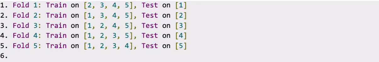
Cross-validation breaks your data into slices (called “folds”) and rotates through them. Each fold takes a turn being the test set, while all the other folds are used as the training set.

Here’s an example with 5-Fold Cross-Validation:

1. Split the data into 5 equal parts (folds).
2. Train the model on 4 parts (the training set) and test it on the 1 part left out (the test set).
3. Rotate so a different part becomes the test set and repeat until every part has had a turn.

At the end, you calculate the average performance across all folds. That’s how well your model performs in general. No cheating!

Each fold gets the chance to help train and also test. Neat, right?

Coding Cross-Validation with Scikit-Learn

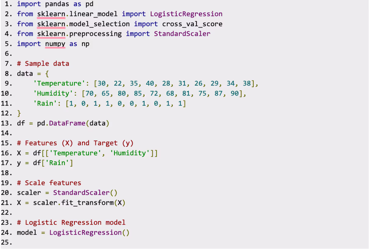
Now, it’s time to see some Python magic! Scikit-learn makes cross-validation super easy. We’ll use the cross_val_score function to test our rain prediction model.

Start by loading your data and model.

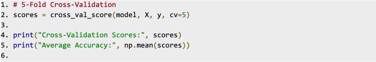
Next, perform Cross-Validation

‍What’s Happening Here?

1. cross_val_score: This function handles the hard part by splitting your data into folds, training the model, and testing it for you.

Parameters:

model- Your logistic regression model.

X- Features (scaled temperature and humidity).

y- Target (rain or no rain).

cv- Number of folds (in this case, 5).

2. scores: This stores the accuracy score for each fold. For example:

3. np.mean(scores): This calculates the average accuracy across all the folds to give you a reliable performance metric:

 This means your model gets rain predictions right about 84% of the time. Not bad!

Why use Cross-Validation?

Here’s why cross-validation is a lifesaver:

• Realistic results: By testing on multiple slices of data, you’re less likely to overestimate how good your model is.
• Avoids randomness: Instead of relying on a single train-test split, cross-validation makes sure every part of the dataset gets its moment in the spotlight.
• Works for small datasets: If you don’t have a ton of data, it ensures you make the most of what you’ve got.

Regularisation

Imagine you’re building a rain prediction model, and it works too well on your training data. It’s so good that it remembers every single detail, but when faced with new weather data, it stumbles. This is called overfitting, and it happens when the model is too complex and focuses on noise or random quirks in the data instead of the big picture.

Regularization is like giving your model some boundaries—helping it stay focused on the patterns that truly matter. It keeps your model from going overboard while still making accurate predictions.

When your model learns, it assigns weights (or importance) to different features. For example, it might decide that “Humidity” is super important for predicting rain and give it a high weight. But sometimes, the model gets carried away and gives extreme importance to every little detail, leading to overfitting.

Regularization stops the model from assigning outrageous weights by applying a penalty. This penalty discourages the model from becoming overly complex. Depending on the type of regularization, it can minimize unnecessary features, reduce their impact, or both.

Think of it as adding a “keep it simple” rule for your model. This way, it performs better on unseen data and avoids being just a memorization machine.

Types of Regularization

There are two main types of regularization in logistic regression:

1. L1 Regularization (Lasso): Shrinks some weights to zero, effectively removing less important features. It’s great for simplifying models.
2. L2 Regularization (Ridge): Reduces the size of weights but doesn’t eliminate them. This keeps all features but controls their impact.

Both types aim to find a sweet spot where the model is neither too simple (underfitting) nor too complex (overfitting). You can even combine them for extra balance, but let's stick with the basics for now.

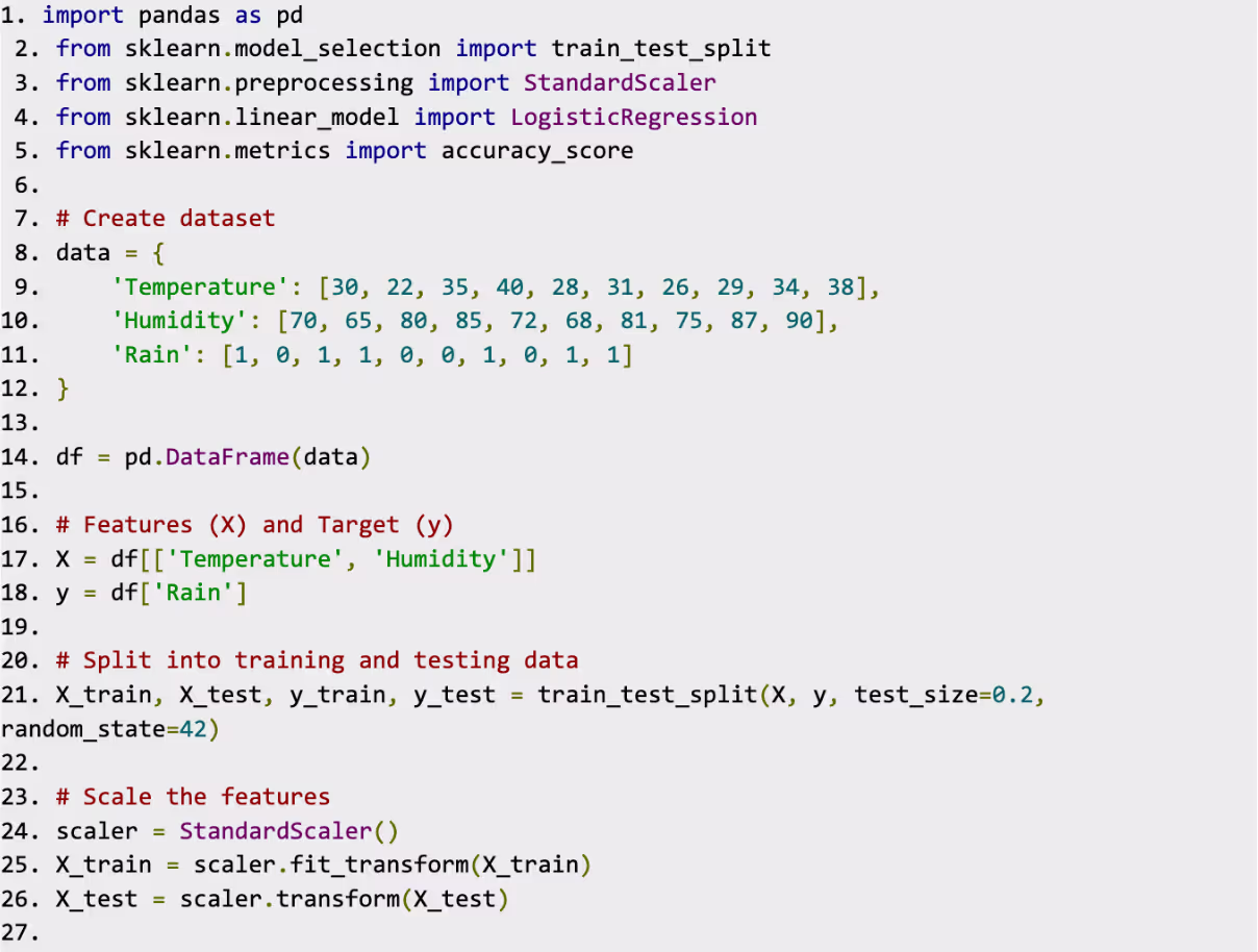
Step 1: Load the Data

Let’s stick with the same example for simplicity.

Step 2: Regularization in Logistic Regression

Scikit-learn makes regularization easy by letting us choose the penalty type (l1 or l2) while creating the logistic regression model. Let's see both in action.

L2 Regularization (Ridge)

By default, logistic regression uses L2 regularization. It prevents overfitting by shrinking the weights but still keeps all features.

Here’s the code:

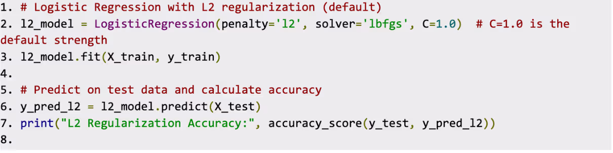
What’s Happening:

1. penalty = 'l2': Tells the model to use L2 regularization.
2. C = 1.0: Controls the strength of regularization. Smaller C means stronger regularization, which adds more penalty to large weights. Larger C does the opposite.

L1 Regularization (Lasso)

L1 regularization takes things further by shrinking some weights to exactly 0, effectively ignoring less important features. To use it, we need a compatible solver like 'liblinear'.

Here’s the code:

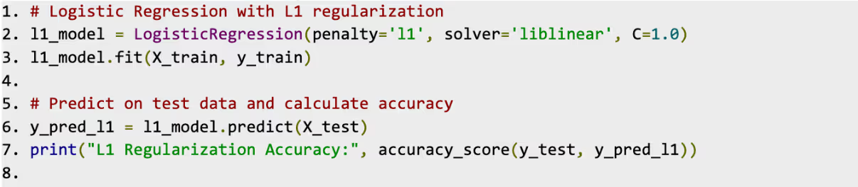
 What’s Happening:

1. penalty = 'l1': Tells the model to use L1 regularization.
2. solver = 'liblinear': Allows for L1 regularization (not all solvers support it).
3. C = Just like in L2, controls regularization strength.

Step 3: Comparing L1 and L2

Here’s a quick summary of what each regularization does when applied to our rain prediction model:

L2 Regularization: Keeps all features but reduces their impact. Use this if you think all your features are important, but you just want to avoid overfitting.

L1 Regularization: Removes less important features by assigning their weights a value of 0. Use this when you have many features and want to simplify your model.

You can also print the coefficients (weights) for each model to see the difference:

If you notice that some coefficients are exactly zero in the L1 model, it means those features were deemed unimportant and removed.

Choosing the Right Regularisation

Choosing between L1 and L2 depends on your data and goals:

1. If your dataset has irrelevant features, L1 might be better for feature selection.
2. If all features are meaningful but you’re worried about overfitting, go with L2.

You can also adjust the regularization strength by tweaking the C parameter:

1. Lower C: Stronger regularization (simpler model).
2. Higher C: Weaker regularization (more complex model).

Accuracy Score

This tells you what percentage of predictions were correct (e.g., 80%).

Confusion Matrix

The confusion matrix helps you see where the model got confused (e.g., predicting rain when it didn’t actually rain).

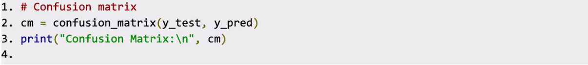
In these two examples, we can see a confusion matrix for binary and multinomial logistic regression models.

Accuracy, Precision, Recall, and F1-Score

Sometimes, you need a more detailed report on how well your model is performing—like whether it’s better at catching the rain or avoiding false alarms. That’s where Accuracy, Precision, Recall, and F1-Score come in.

In the above images, we can see how the confusion matrix for multinomial regression can be “simplified” into binary form. Also note the formulas.

Accuracy: How often is the model correct?

Precision: When the model says “Yes,” how often is it right?

 Recall (Sensitivity): Out of all the actual “Yes” cases, how many did the model catch?

F1-Score: A balance between Precision and Recall.

ROC Curve and AUC

ROC

ROC stands for Receiver Operating Characteristic curve (fancy name, right?). But think of it like a test report that shows how good your model is at telling "Yes" from "No."

The curve plots two things:

1. True Positive Rate (Recall): How many “Yes” cases your model catches.
2. False Positive Rate: How often your model says “Yes” when it’s a “No.”

Imagine testing a metal detector at an airport. You want it to catch all weapons (true positives) while minimizing false alarms like a belt buckle triggering it.

On the ROC curve, if the line is closer to the top-left corner, your model is doing a great job. If it’s just a diagonal line (random guesses), well... time to get back to work improving it!

AUC

AUC stands for Area Under the Curve. It’s like a score for the ROC curve. The higher the AUC, the better your model is overall.

1. 1.0 (Perfect): Your model is a superstar—zero mistakes!
2. 0.5 (Terrible): It’s guessing randomly, like flipping a coin.
3. Below 0.5 (Really bad): The model is worse than guessing and might be upside down.

This simple image can help you visualise the two:

Bring it Together

Let’s see how we can show accuracy, precision, recall and F1-score using Cross-Validation:

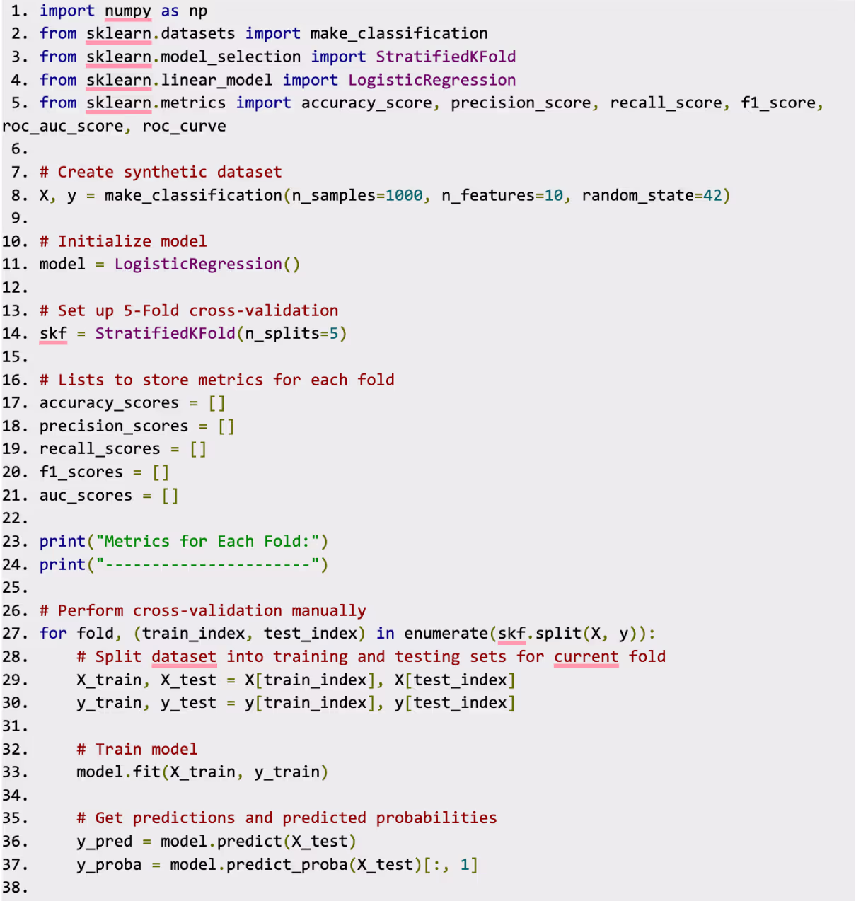
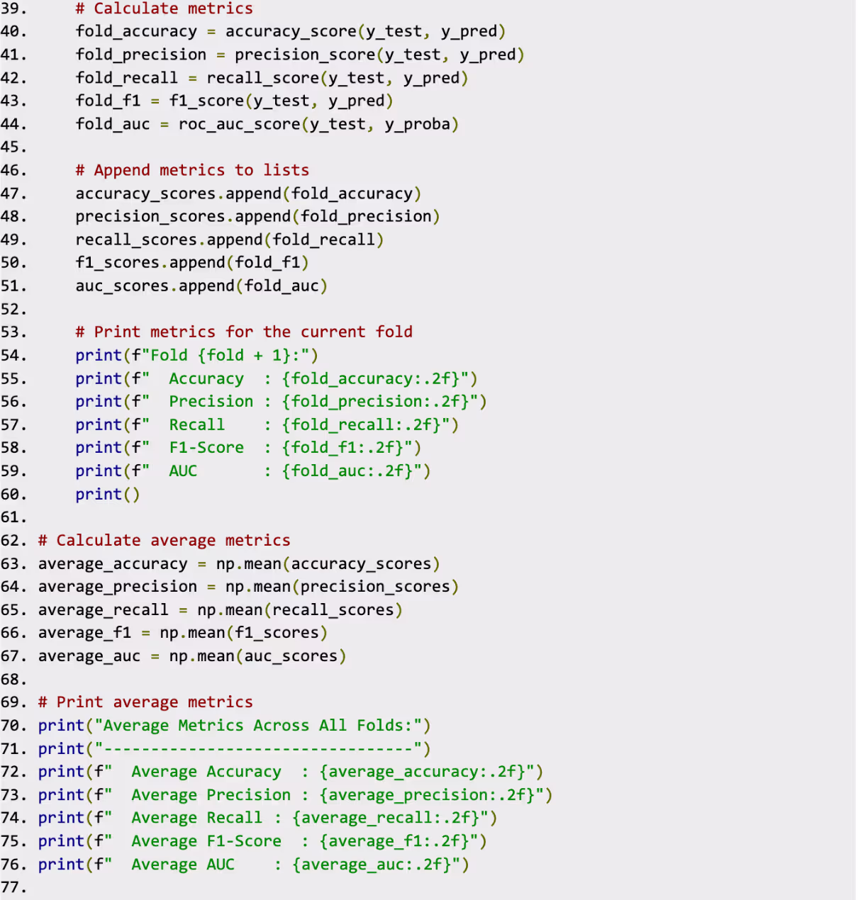
Sample Output:

After running, the output might look like this (values will vary depending on the dataset and model):

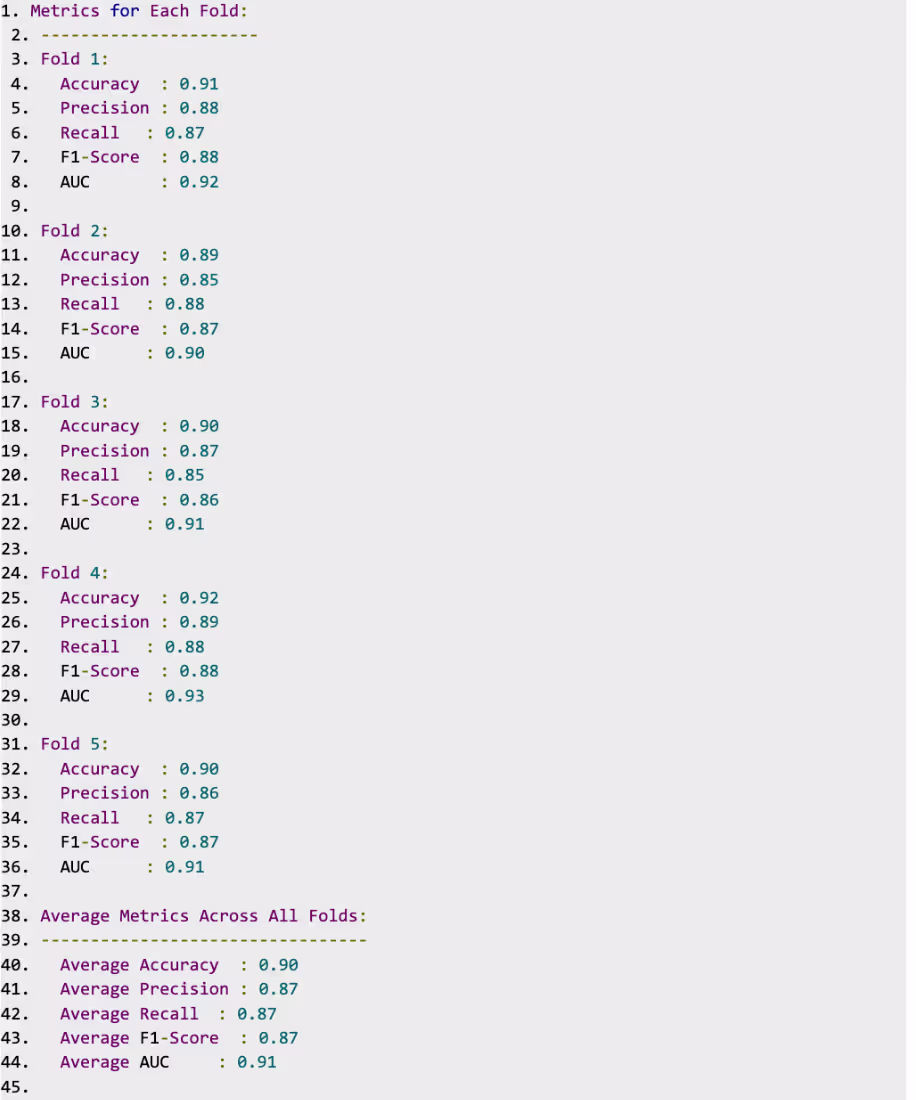
 This approach provides a comprehensive view of the model’s performance across multiple folds!

Conclusion

And that's a wrap on evaluating logistic regression! To sum it up, this model is a fantastic tool for predicting outcomes, but understanding how well it's performing is the real game changer. Metrics like accuracy tell you how often the model gets it right overall, while precision and recall shine a light on how well it's handling specific cases (like catching important positives or avoiding false alarms). The F1 score jumps in when you need a balance between precision and recall, and the AUC helps you see how good the model is at ranking predictions.

The key takeaway? There's no "one-size-fits-all" metric—what you choose should depend on the specific problem you're tackling. For imbalanced datasets, AUC or F1-score might be the superhero you need, while for evenly distributed data, accuracy could do just fine.

Logistic regression is powerful, but it’s only as good as how you measure its performance. By picking the right evaluation tools, you’ll level up your analysis and make smarter decisions with your data. Happy modelling!

‍